SECJ 4423 – Real-Time Software Engineering

📘 Detailed Study Notes (Chapters 5–9)

Companion to the concise summary. This version is organised by chapter → sub-topic so you can revise one sub-topic at a time. Content is drawn only from the official lecture slides (Topic 5 Concurrency, Topic 5 Mechanisms, Topic 7 RTOS, Topic 8 RT Scheduling Parts 1 & 2, and the Utilization/Response-Time worked examples). Redundant duplicate slides were merged; every distinct topic/sub-topic is kept.

📑 Master Table of Contents

Chapter 5 — Introduction to Concurrency

5.1 What is Concurrency

Concurrency = the ability of a system to have multiple tasks in progress at the same time, where the tasks' lifetimes overlap in time.
It is about structure / dealing with many things at once — the tasks need not physically run at the same instant.
Motivation: real-time & embedded systems must handle multiple inputs and control multiple devices simultaneously and reliably (e.g., read sensors while driving actuators while talking to a user).

Need to memorise the definition. "A concurrent program has multiple threads of control that may execute in parallel or be interleaved."

5.2 Concurrency vs Parallelism

Aspect	Concurrency	Parallelism
Meaning	Dealing with many tasks at once (overlapping lifetimes)	Doing many tasks at the exact same instant
Processors	Can be achieved on a single CPU	Requires multiple CPUs / cores
Mechanism	Interleaving	Overlapping
Purpose	Structure, responsiveness	Speed-up, throughput

Key line: parallelism is a way of implementing concurrency, but concurrency does not require parallelism.

5.3 Interleaving vs Overlapping

Interleaving — a single processor rapidly switches between tasks. Only one task actually runs at any instant, but they appear simultaneous → pseudo/semi concurrency.
Overlapping — multiple processors run different tasks at the same real time → true concurrency (parallelism).

5.4 Types of Concurrency (Semi vs True)

Semi (pseudo) concurrency — one processor, achieved by interleaving / time-slicing. Tasks share the CPU in turns.
True concurrency — multiple processors execute tasks simultaneously.

5.5 Process vs Thread

	Process	Thread
Definition	A program in execution with its own address space	A lightweight unit of execution inside a process
Memory	Separate, isolated memory	Shares the process's memory & resources
Overhead	Heavy (expensive context switch)	Light (fast create/switch)
Communication	IPC (messages, pipes, shared mem set-up)	Directly via shared variables (needs sync)
Term for "many"	Multiprogramming	Multithreading

Threads are cheaper but more dangerous — because they share memory, they can corrupt each other's data without synchronisation.

5.6 Sequential vs Concurrent Program

Sequential program — a single thread of control; statements execute strictly one after another in a defined order. Behaviour is deterministic.
Concurrent program — multiple threads of control; parts may be interleaved or run in parallel. Behaviour can be non-deterministic.

5.7 Concurrent System vs Concurrent Program

Concurrent program = the software describing cooperating tasks.
Concurrent system = the execution environment (hardware + OS + run-time support) that actually runs the concurrent program.

5.8 Nature of Concurrent Systems

Tasks are largely independent, but they must:
Cooperate — coordinate to achieve a shared goal (e.g., producer/consumer).
Compete — contend for shared resources (memory, devices, buses).
Execution order between independent tasks is non-deterministic (not fixed by the programmer).

5.9 The Six Problems in Concurrent Programming

High-yield list — memorise all six with a one-line meaning.

Violating Mutual Exclusion — two tasks enter their critical section together and access shared data at the same time → corrupted/inconsistent data. This is the source of race conditions.
Deadlock — tasks each hold a resource and wait for a resource held by another; a circular wait leaves them all blocked forever.
Starvation / Lockout (slides: indefinite postponement) — a task is perpetually denied a resource it needs (others keep getting in first); it ends up waiting for an event that may never occur.
Transient Error — a timing-dependent, intermittent fault; appears only for certain interleavings, hard to reproduce/debug.
Busy Waiting — a task wastes CPU cycles continuously polling ("spinning") instead of blocking/sleeping until it can proceed.
Unfairness — resource allocation among tasks is not equitable (some tasks systematically favoured).

Race condition (definition): the result of a computation depends on the non-deterministic order/timing in which tasks access shared data → a specific manifestation of violating mutual exclusion.

Chapter 6 — Mechanisms to Support Concurrency

6.1 Two Forms of Concurrency

Hardware concurrency — genuine parallelism from multiprocessor / multi-core hardware (overlapping).
Software (logical) concurrency — created by the OS/RTSS via interleaving on possibly a single CPU.

6.2 Non-Determinism (the echo example)

A shared procedure echo() does: read char → store in shared var → write char out.
If two tasks call echo() and their steps interleave, characters can be lost or duplicated.
Lesson: unsynchronised access to shared data produces unpredictable (non-deterministic) results → this is why mutual exclusion is needed.

6.3 Mutual Exclusion & the Critical Section

Critical Section (CS) / Critical Region = the part of a task's code that accesses a shared resource and must not be executed by more than one task at a time.
Mutual Exclusion (MUTEX) = the property that at most one task is inside the CS at any instant.

General structure of a task using a CS:

        entry section       // request permission to enter
        ┌───────────────┐
        │ CRITICAL      │    // access the shared resource
        │ SECTION       │
        └───────────────┘
        exit section        // release permission
        remainder section   // non-critical code

6.4 Requirements for a Correct MUTEX Solution

Mutual exclusion — no two tasks simultaneously in the CS.
Progress — if the CS is free, a task that wants to enter must be allowed in (a task outside the CS must not block others).
Bounded waiting — a task waits only a finite time (no starvation).
No assumptions about relative task speeds or the number of processors.

6.5 Three Approaches to Mutual Exclusion

Memorise the three + their key keyword/operation.

The slides give three broad ways to satisfy the MUTEX requirements:

Software approaches — algorithms using only ordinary shared variables (e.g., Dekker's / Peterson's algorithm).
Special-purpose machine instructions / hardware support — e.g., an atomic test-and-set instruction, or disabling interrupts.
Operating-system / programming-language support — provides the three high-level mechanisms below: (a) semaphore, (b) monitor, (c) message passing.

The course focuses on the three OS/language mechanisms:

(a) Semaphore

An integer variable accessed only by two atomic operations:
wait() / P() — decrement; if value < 0, the task blocks (used before entering the CS).
signal() / V() — increment; wakes a blocked task (used after leaving the CS).
Binary semaphore (values 0/1) → a mutex lock for the CS.
Counting semaphore → manages N interchangeable instances of a resource.

(b) Monitor

A high-level construct that encapsulates shared data + the procedures that operate on it.
Only one task can be active inside the monitor at a time → mutual exclusion is automatic/implicit.
Uses condition variables with wait (block on a condition) and signal (wake a waiting task).

(c) Message Passing

Tasks synchronise & communicate by send / receive messages — no shared memory required.
Synchronous (blocking) — sender/receiver wait to rendezvous.
Asynchronous (non-blocking) — messages buffered; sender continues.

Mechanism	Key operations	Shared memory?	Level
Semaphore	`wait`/`P`, `signal`/`V`	Yes	Low
Monitor	`wait`, `signal` (condition vars)	Yes (encapsulated)	High
Message passing	`send`, `receive`	No	High

Code sketches — the same critical section, three ways:

(a) Binary semaphore (mutex lock):

semaphore mutex = 1;              // binary semaphore, initialised to 1

void task(void) {
    /* ... non-critical code ... */
    wait(mutex);                 // P — block if another task is inside
        /* CRITICAL SECTION: access the shared resource */
    signal(mutex);               // V — release; wake a waiting task
    /* ... remainder ... */
}

Counting semaphore (N interchangeable resource units):

semaphore slots = N;             // e.g. N identical buffers/printers
wait(slots);                     // take one unit (blocks when 0 left)
    /* use one unit of the resource */
signal(slots);                   // return the unit

(b) Monitor (mutual exclusion is automatic; coordinate with condition variables):

monitor BoundedBuffer {
    int count = 0;               // shared state, encapsulated
    condition notFull, notEmpty; // condition variables

    procedure insert(item x) {
        if (count == N) wait(notFull);   // block until space
        /* ... add x ... */  count++;
        signal(notEmpty);               // wake a waiting consumer
    }
    procedure remove() {
        if (count == 0) wait(notEmpty);  // block until item
        /* ... take item ... */ count--;
        signal(notFull);                // wake a waiting producer
    }
}   // only ONE task may be active inside the monitor at a time

(c) Message passing (no shared memory — communicate by copying):

// Producer task                 // Consumer task
item = produce();                receive(Producer, &item);   // blocks until a message arrives
send(Consumer, item);            use(item);

6.6 Concurrent Programming Constructs

A concurrent programming language must provide three fundamental facilities (from the slides):

Expression of concurrent execution — a way to specify concurrent processes (how you launch them).
Process synchronisation — how processes keep shared data consistent.
Interprocess communication — how processes exchange information.

The constructs that provide them:

cobegin … coend (a.k.a. parbegin/parend) — statements between them run concurrently; control passes on only when all finish.
Fork / Join — fork spawns a new thread of control; join waits for it to complete.
PAR — (OCCAM) run processes in parallel; SEQ — run in sequence.

6.7 Concurrent Programming Languages

Language	Concurrency support	Communication model	Notes
Ada	`task`, `PAR`	Rendezvous	Designed for embedded / real-time.
OCCAM	`SEQ`, `PAR`, `ALT`	Channels (message passing, from CSP)	Designed for the transputer.
Java	`Thread` class / `Runnable` interface	Shared memory + monitors	`synchronized`, `wait()`, `notify()`.
Concurrent C-- / BACI	`cobegin … coend`	Shared vars + semaphores	Used in the labs (see Chapter 7).

6.8 Run-Time Support System (RTSS) & Time-Slicing

RTSS = the software layer beneath a concurrent program that manages tasks: creation, scheduling, context switching, synchronisation.
Time-slicing — the RTSS divides CPU time into small slices (quanta) and gives them to tasks in turn → produces logical (semi) concurrency on one CPU.
Context switch — saving the current task's state (registers, program counter, stack pointer) and restoring another task's state so it can resume.

6.9 Two Ways to Achieve Concurrency

Use a concurrent language (Ada / OCCAM / Java) — concurrency is built into the language; its runtime provides the RTSS.
Sequential language + RTOS — e.g., C + µC/OS-II; the RTOS kernel provides tasking. A task is created with a kernel call, e.g.: c OSTaskCreate(TaskFunc, /* pointer to task code */ &task_data, /* argument passed to task */ &TaskStk[SIZE], /* top of the task's stack */ priority); /* task priority */

Chapter 7 — Concurrent Programming in Practice (BACI / jBACI)

7.1 What is BACI / jBACI

BACI = Ben-Ari Concurrent Interpreter — a teaching system for writing and running concurrent programs and observing their behaviour.
jBACI = a Java-based IDE/simulator front-end for BACI that lets you compile, run, and visualise concurrent execution.
Supports Concurrent C-- and Concurrent Pascal dialects.
Purpose in this course: demonstrate non-determinism and race conditions, and show that semaphores/monitors restore mutual exclusion.

7.2 Core Constructs

cobegin p1(); p2(); … coend; — run the listed procedures concurrently.
Semaphore API:
semaphore s; — declare.
initialsem(s, value); — initialise (e.g., 1 for a mutex).
p(s) — wait (enter CS).
v(s) — signal (leave CS).
mutex — a binary-semaphore lock type.

7.3 Counting Possible Outputs (Interleavings)

Because cobegin procedures interleave non-deterministically, the same program can produce different outputs on different runs.
Coarse interleaving (single-core): treat each statement/procedure as an atomic block; the number of possible outputs = the number of distinct orderings/interleavings of those blocks.
Fine interleaving (multi-core): individual operations (read/modify/write of shared vars) can interleave, giving more possible outputs — you trace each step to find the final values.

7.4 Fixing Non-Determinism with Semaphores

Wrap each shared-variable update in a critical section guarded by a binary semaphore initialised to 1: initialsem(mutex, 1); ... p(mutex); // enter CS <update shared variables> v(mutex); // leave CS
Result: updates are serialised → the program produces a single, deterministic output.

Chapter 8 — Real-Time Operating Systems (RTOS)

8.1 What is an RTOS

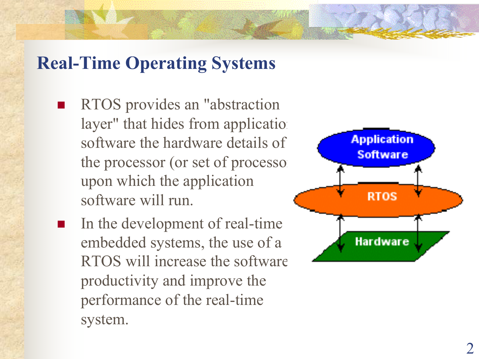
An RTOS provides an "abstraction layer" that hides the hardware details of the processor(s) from the application software.
Correctness depends on logical result AND timing — services must have deterministic, predictable execution times.
Using an RTOS in embedded development increases software productivity and improves real-time performance.
Layer view: Application Software → RTOS → Hardware.

RTOS abstraction layer between Application Software and Hardware — The RTOS is an abstraction layer between application software and hardware, hiding processor details. Topic 7 – RTOS slides

8.2 RTOS vs General-Purpose OS

Four distinguishing points from the slides:

Event-driven scheduling — an RTOS schedules tasks based on external events signalled by interrupts.
Simple command interpreter — few/no utility programs (lean).
Serves the controlled system, not human users — goal is to run the machine, not provide a rich UX.
Deterministic timing — service times are strictly algebraic (no random timing components) to avoid delay and missed deadlines.

	RTOS	General-purpose OS
Goal	Predictability / meeting deadlines	Average throughput & fairness
Scheduling	Priority-based, preemptive, event-driven	Time-sharing / fair-share
Timing	Deterministic, bounded	Best-effort, variable
Users	Serves the system it controls	Serves human users
Size	Small, lean kernel	Large, many utilities

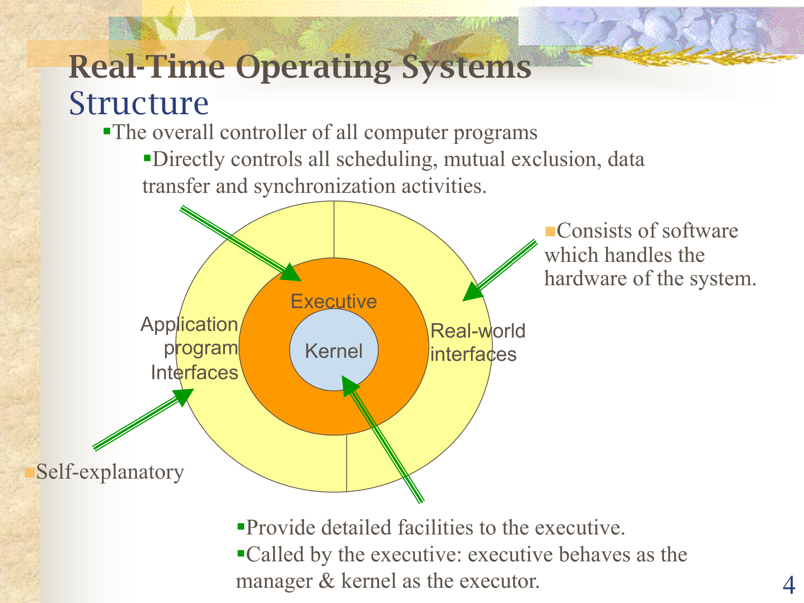
8.3 RTOS Structure (4 Elements)

Exam-relevant: name all four and what each does.

Element	Role
Executive	The overall controller of all programs. Directly controls scheduling, mutual exclusion, data transfer, and synchronisation. Acts as the manager.
Kernel	Provides detailed facilities to the executive; called by the executive. Acts as the executor. (Executive = manager, kernel = executor.)
Application Program Interfaces (APIs)	Interface through which application software requests OS services (self-explanatory).
Real-World Interfaces	Software that handles the hardware of the system (talks to sensors/actuators/devices).

RTOS structure: Executive wraps the Kernel, with APIs and Real-world interfaces — The **Executive** (manager) surrounds the **Kernel** (executor); **APIs** face the application, **Real-world interfaces** face the hardware. Topic 7 – RTOS slides

8.4 RTOS Basic Services

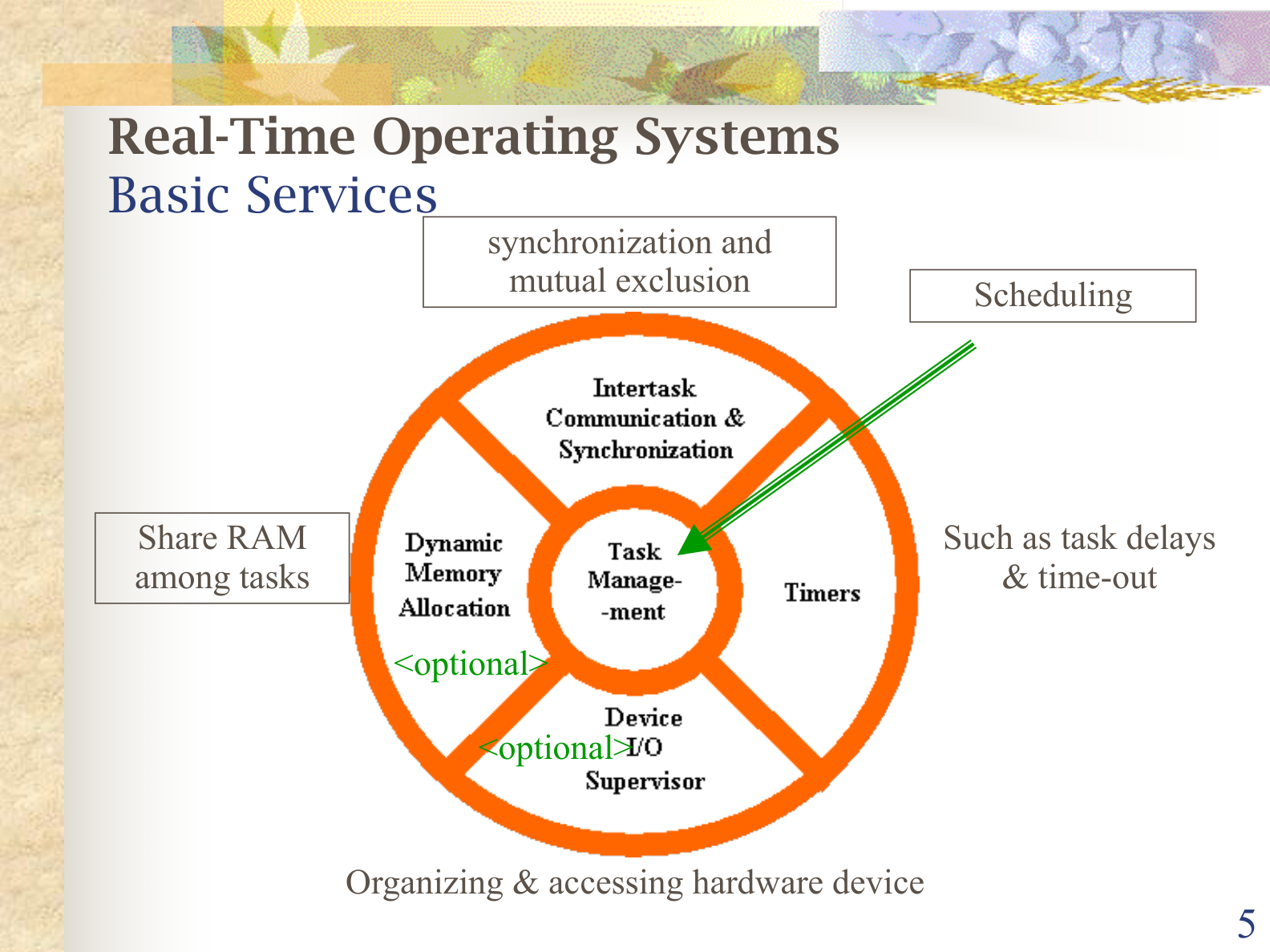
Central service is Task Management; surrounding services:

Task Management — lets developers split software into separate tasks ("chunks"); the main job is scheduling tasks at run time so they run in a timely, responsive way.
Intertask Communication & Synchronisation — lets tasks pass information safely (without corruption) and coordinate/cooperate.
Timers — services such as task delays and time-outs.
Dynamic Memory Allocation (optional) — tasks "borrow" RAM chunks temporarily; can pass memory task-to-task to move large data quickly. Very small kernels omit this.
Device I/O Supervisor (optional) — organising & accessing hardware devices.

RTOS basic services arranged around Task Management — RTOS basic services arranged around the central **Task Management**: Intertask Communication & Synchronisation, Timers, Dynamic Memory Allocation*, Device I/O Supervisor* (*optional). Topic 7 – RTOS slides

8.5 Example RTOSs

Micrium µC/OS-II, AvrX, RTLinux, QNX Neutrino.

8.6 µC/OS-II Introduction & Features

µC/OS-II = Micro-Controller Operating System, Version 2 (based on µC/OS 1.0, 1992); targeted at embedded systems.

Features (memorise the list):

Feature	Meaning
Portable	Mostly ANSI C; only tiny CPU-specific part in assembly. Runs on 8/16/32/64-bit MCUs & DSPs (needs a stack pointer + push/pop of CPU registers).
ROMable	Designed to be embedded in ROM as part of the product.
Scalable	Use only the services you need → reduces RAM/ROM (code & data space).
Preemptive multitasking	Fully preemptive; always runs the highest-priority ready task. Manages up to 64 tasks (8 reserved for system).
Deterministic	Execution time of every function/service is known & bounded.
Task stacks	Each task has its own stack; sizes can differ; stack-checking feature measures actual usage.
Services	Mailbox, queue, semaphore, time functions, etc.
Interrupt management	Interrupts can suspend/resume tasks; can be nested up to 255 levels.
Robust & Reliable	Field-proven in cameras, medical/musical instruments, engine controls, ATMs, industrial robots, etc.

8.7 µC/OS-II Architecture

Layered top→bottom:

┌─────────────────────────────────────────────┐
│              Application Software            │   ← your tasks
├───────────────────────┬─────────────────────┤
│  µC/OS-II             │  µC/OS-II Config     │   Software
│  (MP-Independent)     │  (Application-Specific)│
├───────────────────────┴─────────────────────┤
│      µC/OS-II PORT  (Microprocessor-Dependent)│  ← the porting layer
├──────────────────────────────────────────────┤
│        Microprocessor   |    Timer            │   Hardware
└──────────────────────────────────────────────┘

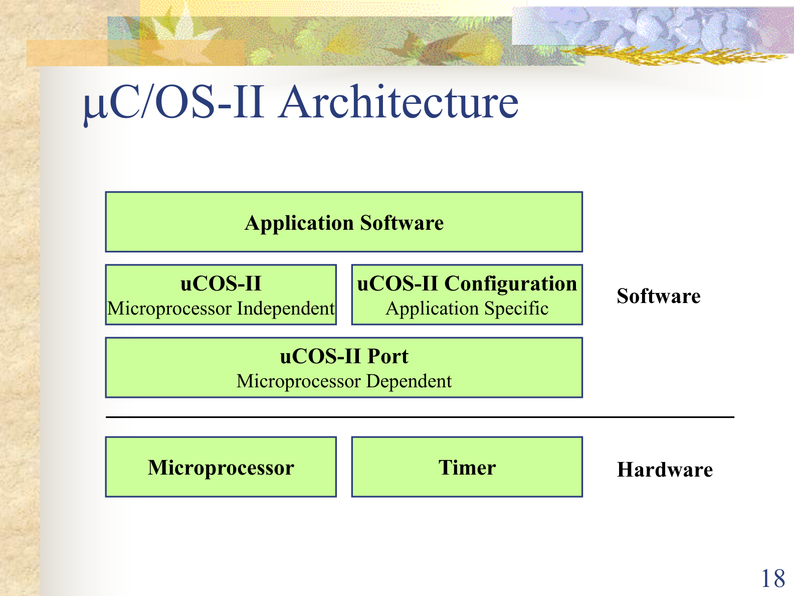
uC/OS-II architecture layers — µC/OS-II architecture — Application Software over the MP-independent core + Configuration; the **Port** (MP-dependent) below; then Microprocessor + Timer hardware. Topic 7 – RTOS slides (cf. exam Figure A4.2)

µC/OS-II (MP-independent): the portable core kernel (same on every CPU).
µC/OS-II Configuration (application-specific): compile-time options selecting which services/limits are included.
µC/OS-II Port (MP-dependent): the hardware-specific glue — code that adapts the kernel to a particular microprocessor (context-switch, stack init, timer/tick hook). Function of the Port = make the portable kernel run on a specific CPU. This is what you rewrite when moving to new hardware.
Hardware: the microprocessor + timer that generates the clock tick.

Chapter 9 — Real-Time Scheduling & Schedulability Analysis

9.1 What is Scheduling

Scheduling = deciding the order and timing in which ready tasks use the processor so that all timing constraints (deadlines) are met.
Goals: meet all deadlines, keep the system predictable, use the processor efficiently, minimise response time.

9.2 Task Model & Parameters

Symbol	Name	Meaning
T	Period	Time between successive releases of a periodic task
D	(Relative) Deadline	Time by which a task must finish after release (often D = T)
C	Computation time (WCET)	Worst-Case Execution Time
R	Response time	Release → completion time (compare to D)
a / S	Arrival / start time	When the task is released
U	Utilization	Fraction of CPU a task needs = C / T

9.3 Task Types

Periodic — released at fixed regular intervals (period T). Typically hard deadlines.
Aperiodic — irregular/random arrival; usually soft deadlines.
Sporadic — irregular arrival but with a guaranteed minimum inter-arrival time; typically hard deadlines.

9.4 Classification of Scheduling

Independent axes you can mix & match:

Pre-run-time (offline / static) vs Run-time (online / dynamic) — when the scheduling decision is made.
Fixed priority (priority never changes, e.g., RM) vs Dynamic priority (priority changes at run time, e.g., EDF).
Preemptive (a higher-priority ready task can interrupt a running lower-priority task) vs Non-preemptive (a running task runs to completion before another starts).
Non-preemptive fixed-priority (key characteristic): once a task starts it cannot be interrupted; a newly-arrived higher-priority task must wait until the current task finishes → simpler, but causes priority-inversion-like blocking.

9.5 Basic Scheduling Policies

The slides (Cooling) list four basic policies: cyclic, time-slicing, task priorities, and using queues.

Cyclic (cyclic executive) — a fixed, repeating timeline of slots; computed offline. Very predictable, but inflexible.
Time-slicing / Round-Robin — equal CPU quanta rotated among ready tasks; fair but not deadline-aware.
Task priorities (priority-based, preemptive) — always run the highest-priority ready task; it may preempt lower-priority tasks.
Using queues — ready tasks are held in queues (e.g., one ready-queue per priority level, plus delay/timer queues); the scheduler dispatches from the head of a queue. This is the underlying mechanism the other policies are built on.

9.6 Rate Monotonic (RM)

Fixed-priority policy.
Rule: the shorter the period T, the higher the priority (higher rate → higher priority).
Priorities assigned once, offline.
Optimal among all fixed-priority algorithms.

9.7 Earliest Deadline First (EDF)

Dynamic-priority policy.
Rule: the task with the earliest absolute deadline runs next; priorities recomputed at run time.
Optimal among all scheduling algorithms; can reach 100% utilization.

9.8 RM vs EDF

	Rate Monotonic (RM)	Earliest Deadline First (EDF)
Priority type	Fixed / static	Dynamic
Priority rule	Shorter period → higher priority	Earliest deadline → higher priority
Assigned	Offline (once)	At run time (recomputed)
Utilization bound	n(2^(1/n) − 1) (→ 0.693)	1 (100%)
Optimality	Best among fixed-priority	Best among all algorithms
Overhead	Low, simple	Higher (track deadlines)
Predictability under overload	Degrades gracefully (low-priority misses)	Can cascade (domino effect)

9.9 Priority Inversion & Priority Inheritance

Listed in the official RTS-concepts revision slide and used in problem-solving. Know the definitions and the fix.

Priority Inversion — a high-priority task is blocked waiting for a resource held by a low-priority task. If a medium-priority task then preempts the low-priority holder, the high-priority task is delayed indirectly by an unrelated medium task → its effective priority is "inverted."
Priority Inheritance (the fix) — while a low-priority task holds a resource needed by a high-priority task, it temporarily inherits the high task's priority. This stops medium-priority tasks from preempting it, so it releases the resource sooner, and the high-priority task resumes with bounded blocking.
Priority Ceiling Protocol — a stronger fixed-priority resource protocol named in the slides (RM + priority-ceiling). Each resource is given a ceiling = the priority of the highest-priority task that can lock it; a task may lock a resource only if its priority is higher than the ceilings of all resources currently locked by other tasks. It prevents deadlock and bounds blocking to at most one critical section.

9.10 Schedulability Analysis — Overview

Schedulability Analysis (SA) = determining whether a set of tasks can be scheduled so every task meets its deadline under a given algorithm.
A Schedulability Test (ST) validates this. (With resource dependencies the general problem is NP-hard.)
Three basic approaches: 1. Processor Utilization Analysis (ST1 EDF, ST2 RM) 2. Processor Workload Analysis (ST3) 3. Response Time Analysis (ST4)

9.11 ST1/ST2 — Processor Utilization Analysis

ST1 — EDF (Dᵢ ≥ Tᵢ; periods integer multiples). Necessary & sufficient:

U = Σ_i=1ⁿ (C_i)/(T_i) ≤ 1

ST2 — RM. Sufficient condition (Liu & Layland):

U = Σ_i=1ⁿ (C_i)/(T_i) ≤ n(2^1/n - 1)

Utilization bound U(n):

n	1	2	3	4	5	→ ∞
U(n)	1.000	0.828	0.779	0.756	0.743	0.693

Interpretation: if U ≤ U(n) → schedulable (guaranteed). If U > U(n) under RM → inconclusive (the test is only sufficient); use Response Time Analysis to decide.
How to apply: compute each Uᵢ = Cᵢ/Tᵢ, sum them, compare against U(n) for the number of tasks n.
⚠️ Slide wording: the lecture slide labels ST2 (RM) as "necessary & sufficient." In practice treat the RM utilization bound as sufficient only — when U exceeds it the result is inconclusive, not "unschedulable." That is exactly why the workload (ST3) and response-time (ST4) tests are provided, and why the class exercise re-checks a task with RTA even after the utilization test.

9.12 ST3 — Processor Workload Analysis

ST3 — RM. Task Jᵢ is schedulable iff the cumulative workload catches up with time at some instant:

W_i(t) = Σ_k=1ⁱ C_k ⌈ (t)/(T_k) ⌉, 0 < t ≤ T_i

The test passes if Wᵢ(t) ≤ t for some t taken from the set:

t = k T_j, j = 1… i, k = 1 … ⌊ (T_i)/(T_j) ⌋

If Dᵢ ≠ Tᵢ, replace Tᵢ with min(Dᵢ, Tᵢ).
Uses ceiling ⌈⌉ inside the sum and floor ⌊⌋ to bound the candidate instants.

9.13 ST4 — Response Time Analysis

ST4 — RM. Task i is schedulable if Rᵢ ≤ Dᵢ, where Rᵢ is the fixed point of:

R_i^x+1 = C_i + Σ_{j ∈ hp(i)} ⌈ (R_i^x)/(T_j) ⌉ C_j

hp(i) = the set of tasks with higher priority than i (shorter periods, under RM). Only these cause interference.
The second term = interference from higher-priority tasks preempting i.

Iterative algorithm (memorise the 3 stop conditions):

Step 1 — first approximation: a₀ = Σ Cⱼ (C of task i plus all higher-priority tasks).
Step 2 — next approximation: plug aₙ into the recurrence to get aₙ₊₁.
Step 3 — decide:
Condition 1: aₙ₊₁ ≤ Dᵢ AND aₙ₊₁ ≠ aₙ → repeat Step 2.
Condition 2: aₙ₊₁ > Dᵢ → the task misses its deadline (not schedulable).
Condition 3: aₙ₊₁ = aₙ → converged; aₙ is the response time (WCRT). Schedulable if ≤ Dᵢ.

Why RTA matters: it is exact (necessary & sufficient) for fixed-priority preemptive scheduling — so a task set that fails the utilization test may still be proven schedulable by RTA.

End of detailed notes. Every distinct sub-topic from the official Ch5–9 slides is included; duplicated slides were merged. For practice questions see MCQ_Bank.html; for exam-focus guidance see Exam_Topic_Map.md.